How to Choose the Cam Curve Form of Zoom Lenses?
- Share
- Issue Time
- Nov 5,2021
Summary
Cam curve design is an indispensable step in the optimization design of infrared zoom lenses. This article will select the appropriate cam curve form of the zoom lens through examples and analysis.
In the final stage of the zoom lens design, the cam curve needs to be designed. In order to balance the uniformity of the imaging magnification change and the cam rotation angle, a suitable cam curve form needs to be selected, and a certain functional relationship between the imaging magnification M and the cam rotation angle θ must be established.
According to the actual boundary conditions and function continuity to be met by the cam curve, several common functional relations between M and θ are established, and the design examples are simulated by Matlab.
The results show that when the established power function relationship between the imaging magnification M and the cam rotation angle θ and the pressure rise angle does not exceed the allowable value, the variable magnification change balance is the best, the magnification change curve is smooth, and there is no cam inflection point. This method can facilitate designers to change the cam curve shape according to different design requirements and find the best zoom cam curve.
In the zoom system, the cam is the component that controls the movement of the lens group and enables the system to change the focal length while keeping the image plane stable. The smooth, flexible, and fast zoom operation is an important content of the zoom performance, which is directly related to the roughness of the cam profile and the pressure angle of the cam curve.
If the cam curve has a larger inclination angle in a certain section, it appears steeper. In the process of rotating the cam, there will be a heavier hand feeling. The gear that drives the cam to rotate is worn out, and the edge of the cam groove may even be squeezed and deformed, which affects the imaging quality; when it is more serious, the cam will be stuck and cannot be used at all.
In the mechanically compensated zoom lens, by selecting the movement relationship between the movement of the zoom group and the cam angle, it can be satisfied that the imaging magnification changes at a uniform speed or at a uniform acceleration during the zooming process. This is very promising whether it is for television, film photography, or zoom lenses used in military tracking.
But at the same time, the pressure angle corresponding to the cam curve at both ends of the long and short focal lengths will be very large. When pursuing the miniaturization of the zoom lens, the rotation torque of the cam will often exceed the tolerable value. Therefore, it is necessary to choose the cam curve form and find a balance between the uniformity of the imaging magnification change and the cam rotation angle.
This paper establishes the power function relationship between the imaging magnification M and the cam rotation angle θ. Combined with the zoom system equation, the Matlab simulation interface is written to simulate the cam curve form. The results show that the established function M-θ is more linear than the traditional curve fitting and θ-x Method, the cam curve is smoother, the pressure rise angle is smaller overall (<45°), and the magnification change is more balanced.
The basic theory of the zoom system
The final stage of zoom lens design, that is, after the optical mechanism parameters (radius, interval, glass material) of each lens element is determined, it is also necessary to calculate the numerical relationship between the displacement of the zoom group and the compensation group to process the cam track. Below we discuss the two forms of the cam curve equation.
Form 1: Obtain the compensation group movement amount y from the variable magnification group movement amount x, and then obtain the variable magnification cam curve, namely
x→y→m2* ,m3* →M (1)
Form 2: Obtain the magnifications m2* and m3* of the variable magnification group and the compensation group from the variable magnification M required by the system, and obtain the movement x, y of the variable magnification group and the compensation group, and then obtain the cam curve, namely
M→m2*,m3*→x,y (2)
It can be seen from the above two forms that in order to establish the cam equation and then process the cam track, it is necessary to establish the functional relationship between the cam angle and one of the above variables.
Design of zoom cam curve
In order to balance the uniformity of the imaging magnification change and the cam angle, it is necessary to select a suitable cam curve form. This requires us to establish a certain functional relationship between the imaging magnification M and the cam rotation angle θ, which will be discussed below.
1. Formal discussion
First, specify the following symbols.
f1,f2,f3,f4: They are the focal lengths of the front fixed group, zoom group, compensation group, and rear fixed group;
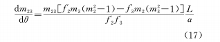
m2,m3: Respectively the lateral magnification of the zoom group and the compensation group;
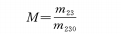
m23=m2m3: The lateral magnification of the variable magnification part composed of the variable magnification group and the compensation group;
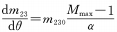
m230:The horizontal magnification of the variable magnification part at the starting point (θ=0) at the focal position. This example is the shortest focal length position;
L: The maximum movement of the zoom group;
θ:The rotation angle of the cam;
α:The maximum rotation angle of the cam;
R: Drum radius:
M: Zoom magnification;
Max: Maximum zoom magnification;
x,y: Respectively represent the movement amount of the zoom group and the compensation group;
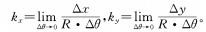
Among them, kx and ky are the slopes of the cam curve zoom group and the compensation group respectively, that is, the tangent value of their pressure rise angle.
When constructing the functional relationship between θ and M, two boundary conditions need to be paid attention to:
Boundary condition one: When θ=0°, M=1
Boundary condition two: When θ=α, M=Mmax
(1) θ has a linear relationship with M
It can make the magnification change produce a uniform effect, this relation can be expressed as
The above formula can be used to differentiate θ to obtain the rate of change of magnification:
(1) There is a linear relationship between θ and M
(a) First construct the power function relationship between θ and M:
M: Zoom magnification;
Mmax: Maximum zoom magnification;
x,y: Respectively represent the movement amount of the zoom group and the compensation group;
Among them, kx and ky are the slopes of the cam curve zoom group and the compensation group respectively, that is, the tangent value of their pressure rise angle.
When constructing the functional relationship between θ and M, two boundary conditions need to be paid attention to:
Boundary condition one: When θ=0°, M=1
Boundary condition two: When θ=α, M=Mmax
(1) θ has a linear relationship with M
It can make the magnification change produce a uniform effect, this relation can be expressed as

The above formula can be used to differentiate θ to obtain the rate of change of magnification:
(1) There is a linear relationship between θ and M
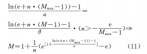
(a) First construct the power function relationship between θ and M:
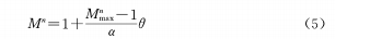
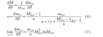
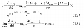
In the formula, M, Mmax, α, θ are defined as above, n is the cam curve coefficient, which can also be regarded as an adjustment coefficient, and n≠0 is specified. (5) Differentiating the formula to θ can be obtained:
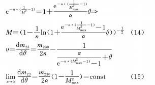
(b) Construct the exponential function relationship between θ and M
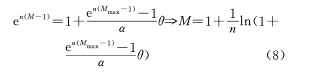
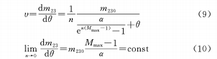
The formula (8) can be obtained by differentiating θ:
(c) Construct the logarithmic function relationship between θ and M
After differentiation, there is
(d) Construct the Gaussian function relationship between θ and M
(e) The above four functional relationships are used in the case of n≠0. For the case of n=0, we stipulate:
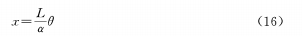
That is, there is a linear relationship between θ and x, which is currently the most commonly used relationship. Differentiate equation (16) and the cam equation to obtain the rate of change of the magnification as
The above results are discussed below.
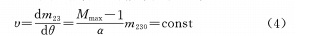
(1) When θ has a linear relationship with M, it can be seen from the formula (4) that the system variable times and uniform speed are very desirable. However, due to the non-linear relationship between the movement amount x of the zoom group and M, it will inevitably lead to the non-uniformity of the movement speed of the lens group and the imbalance of the pressure angle.
(2) When θ and M are in a non-linear relationship, and θ and M are in a backup function relationship, if n is constant, the variable magnification and the rotation angle will change in a backup function relationship. It can be seen from the formula (7) that when the cam curve coefficient n approaches 0, the variable magnification and the rotation angle change exponentially, that is, the magnification increases faster and faster during the cam rotation.
When n=1 and the conditions of the above formula appear, the rate of change of magnification is a fixed value, that is, during the entire rotation of the cam from the end of the shortest focal length to the end of the longest focal length, the change of magnification is uniform, which becomes the situation discussed in formula (4).
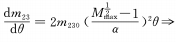
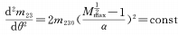
When m=1/2 and the conditions of the above formula appear, so the magnification change is uniformly accelerated, which is also what we expect.
(3) The relationship between θ and M is exponential, logarithmic, and Gaussian. When n is constant, the rate of change of magnification is inversely proportional to θ, that is, when the cam gradually rotates from the shortest focal length to the longest focal length, the rate of change of magnification becomes slower and slower.
When n changes, the rate of change of magnification is nonlinear with the θ curve. When the cam curve coefficient n approaches 0, the rate of change of the magnification is a constant, that is, the change of the magnification is linear.
Generally speaking, the principle of selecting the cam curve is to select the curve form with the best variable magnification change and smooth magnification change curve when the pressure rise angle does not exceed the allowable value.
Through the above discussion and Matlab experimental simulation, we understand that when the relationship between θ and M is a backup function, by selecting the appropriate adjustment coefficient n, it can be achieved that when the pressure angle is close to the allowable value, the variable magnification change has the best balance and the magnification change. The curve is smooth and there is no cam inflection point.
However, none of the other functions can achieve better results. Figure 1 is a cam simulation diagram designed using three-dimensional drawing software based on the previous analysis results. The following describes the results of our simulation experiments.
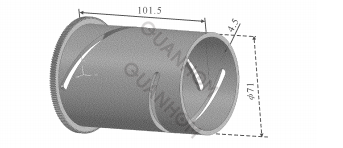
Fig. 1 Simulation figure of cam
2. Analysis and simulation
Combine the two forms of cam curve solving methods given above, and the functional relationship between θ and M, to compile the Matlab GUI interface.
The program input parameters are:
Cam curve coefficient n, optical system's short focal length f0, variable magnification group focal length f2, compensation group focal length f3, lead (movement distance of the variable magnification group from short focal length to long focal length) wl, objects in the variable magnification group at short focal length, the distance is l20, the image distance of the compensation group is ll30 at short focus, the maximum cam rotation angle α, the rotation angle interval mu in angle units, and the diameter of the cam drum dd.
The program output parameters are:
Rotation angle, movement of the zoom group, movement of the compensation group, focal length, pressure rise angle of the zoom group, pressure rise angle of the compensation group, and zoom ratio data and graphics.
Through this program interface, you can easily see the relationship between the zoom ratio and the angle of rotation, observe whether the pressure rise angle exceeds the allowable value, and change the adjustment coefficient to quickly change the above relationship to find the best cam curve required.
Take the 20X continuous zoom positive compensation system designed by the research group as an example to select the cam curve.
The fixed parameters are:
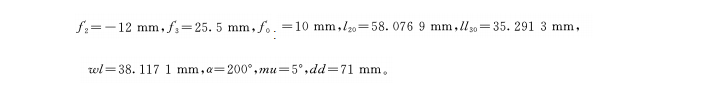
Variable parameter: adjustment coefficient n
This program is editable for all the above parameters. In order to facilitate the discussion, here we mainly consider the influence of the adjustment coefficient n on the result.
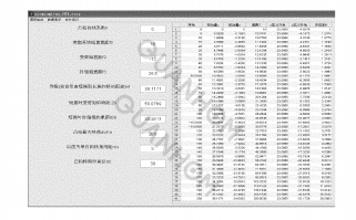
Fig. 2 Matlab simulation interface
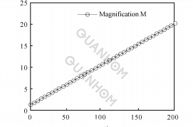
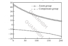
(1) When n=0, there is a linear relationship between θ and x, as shown in Figure 3.
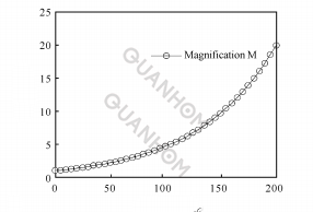
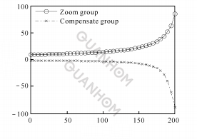
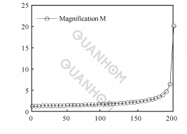
(2) When n = 0. 047, the power function graph is shown in Figure 4.
(3) When n= 0. 000 1, the graph of the exponential function is shown in Figure 5.
(4) When n= 2.32, the logarithmic function graph is shown in Figure 6
(5) When n = 0.1, the graph of the Gaussian function is shown in Figure 7.
The experiment proves that the previous discussion on the relationship of various functions is consistent with the trend of the graph curve.
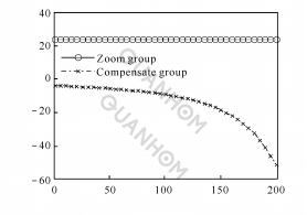
(a)Relationship between pressure rise angle and rotation angle
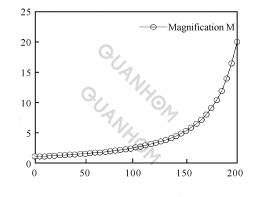
(b) Relationship between zoom ratio and rotation angle
Fig. 3 Linear relationship between θ and x
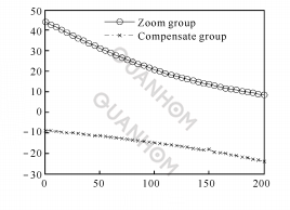
(a)Relationship between pressure rise angle and rotation angle
(b) Relationship between zoom ratio and rotation angle
Fig. 4 Power function between θ and M
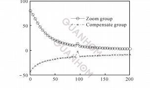
(a)Relationship between pressure rise angle and rotation angle
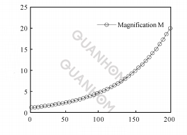
(b) Relationship between zoom ratio and rotation angle
Fig. 5 Exponential function between θ and M
(a)Relationship between pressure rise angle and rotation angle
(b) Relationship between zoom ratio and rotation angle
Fig. 6 Logarithm function between θ and M
(a)Relationship between pressure rise angle and rotation angle
(b) Relationship between zoom ratio and rotation angle
Fig. 7 Gauss function between Q and M
The above example analysis briefly illustrates the influence of different values of the adjustment coefficient n on the design results of the cam curve, and the appropriate modification of the parameters can obtain better results.
During the test, it was found that when n takes certain specific values, the overall pressure angle of the cam curve meets the requirements, and only a certain point suddenly exceeds a reasonable value. Such a point is what we often call the curve inflection point, which is when the cam rotates. When it reaches a certain angle, it suddenly cannot continue to rotate, that is, it is stuck in the machine.
It is fatal to both the cam structure and the zoom effect, so when designing, you should avoid curves with such inflection points. That is, multiple tests are required to ensure that a reasonable adjustment coefficient is obtained.
At the same time, whether a certain value of the adjustment coefficient can optimize the cam curve is related to the requirements of the diameter of the cam, the pressure angle of the cam curve that it can bear, the requirements of the total cam rotation angle, the volume and weight of the system, and the requirements of the zoom speed.
Therefore, the design method of establishing the zoom cam curve equation of the adjustment coefficient can facilitate designers to modify the curve flexibly, so that they can change the shape of the cam curve according to different design requirements and find the best zoom cam curve.
Randomly take out several zoom positions from the above experimental data and bring them to Code V to verify that the image surface is stable and the image quality meets the design requirements.
3. Experimental results
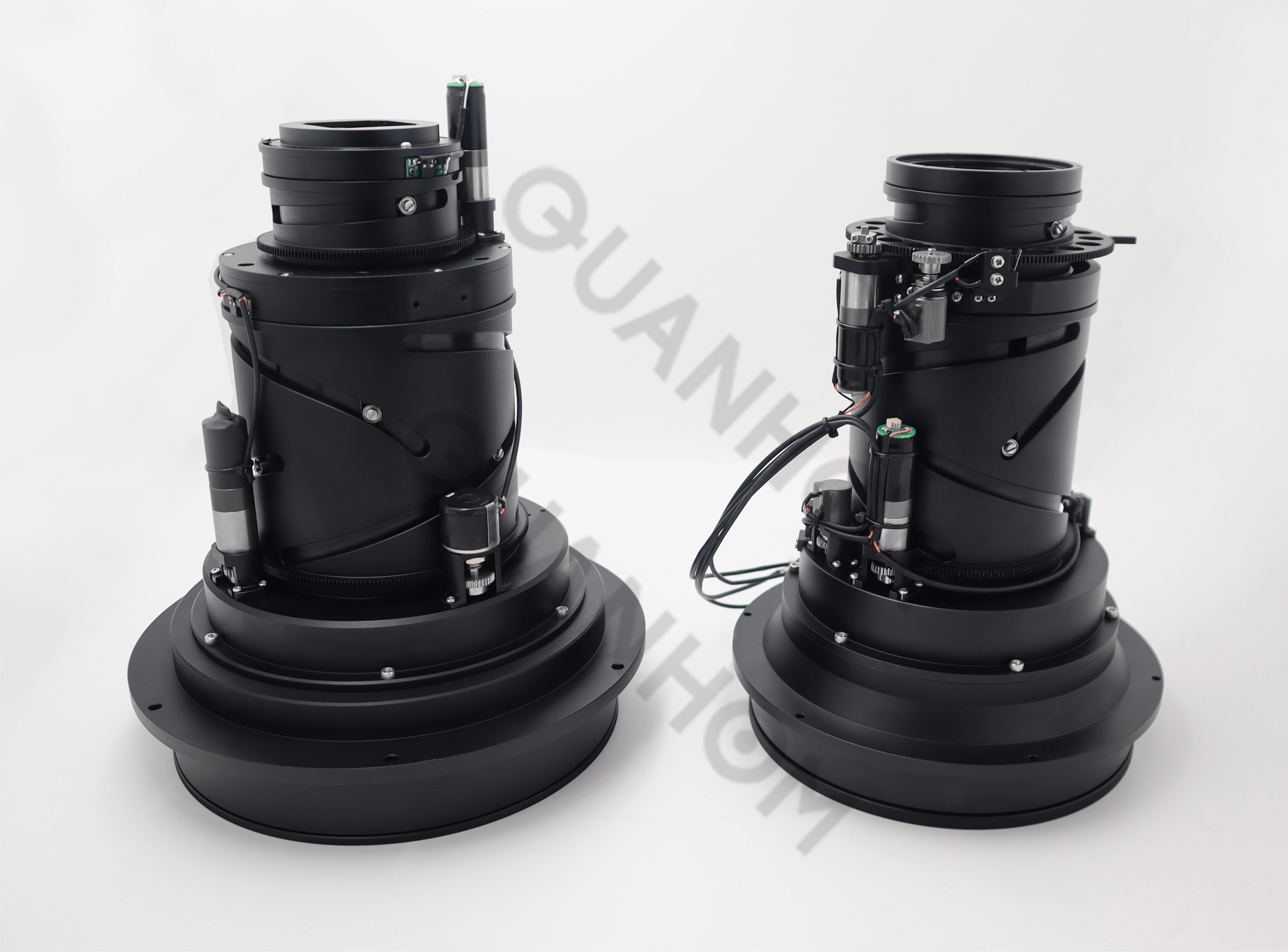
According to the above analysis and simulation, the cam of the zoom lens we designed has been successfully applied, as shown in Figure 8. After field photography inspection, the cam designed using the above theory in the zoom lens has fast and smooth zoom, accurate compensation curve, good image quality at different focal points, and fully meets the design indicators, which verifies the correctness of the foregoing analysis.
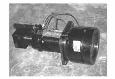
Fig. 8 Zoom lens
Select the power function relationship between θ and M, and by changing the adjustment coefficient n, different compromises can be made between the linear relationship between θ and x and the linear relationship between θ and m23, which not only ensures that the pressure rise angle will not be too large but also avoid to overcome the serious non-uniformity of the rate change speed.
Of course, in order to obtain a linear relationship of θ-m23 or θ-dm23/dθ, you can increase the α angle or increase the diameter of the cam drum to reduce the maximum pressure rise angle of the cam curve, but this will increase the volume and weight of the lens. Decreasing the focal length of the compensation group will also reduce the maximum pressure rise angle of the compensation curve.
This will complicate the structure of the fixed group and even reduce the quality of the optical design. Therefore, choosing the power function relationship between θ and M can help us optimize the cam curve and help us design a miniaturized high-quality zoom lens.
If you want to get more information about the zoom lens after reading the above content, you can contact Quanhom for a comprehensive solution.
As a professional manufacturer of Opto-electromechanical components with many years of experience, Quanhom is equipped with a professional R&D team and strict quality inspection system. Our various thermal infrared lenses (LWIR, MWIR, and SWIR cameras) are sold all over the world and have received praise and trust from many customers. We put the needs of customers first in everything and can provide customers with thoughtful customized services. If you want to buy our infrared continuous zoom lens, please contact us immediately!
Authors: Yan Lei, Jia Ping, Hong Yongfeng, Wang Ping
Journal source: Vol.31 No.6 Journal of Applied Optics Nov. 2010
Received Date: 2010-03-25 Revision Date: 2010-6-23
References:
[1] TANG Jian-bing. Optimized design of vari-focus cam contour [J]. Optical Technique, 1994,20(1) : 27- 29. (in Chinese with English abstract)
[2] ZHANG Xiu-li. A new method to improve the cam contour of compensating lens [ J ]. Yunguang Technique, 2003,35 (2): 16-17. (in Chinese with English abstract)
[3] CUI Jun, HE Guo-Xiong. Fitting design of zoom lens cam contour [J]. Chinese Journal of Scientific Instrument, 1990,11 (1) : 107-112. (in Chinese with English abstract)
[4] Movie Lens Design Group. The optical design of movie photography objective lens [ M ]. Beijing: Chinese Industry Publishing Company, 1971. (in Chinese)
[5] CHANG Qun. Optical design corpus [M]. Beijing: Science Publishing Company, 1976. (in Chinese)
[6] CUI Ji-cheng. Design of large aperture refractive- reflective zoom lens [J]. Optics and Precision Engineering, 2008? 16 (11) : 2087-2091. (in Chinese with English abstract)
[7] DONG Ke-yan, PAN Yu-long, WANG Xue-jin, et al. Optical design of an HDE infrared dual-band step-zoom system [ J ]. Optics and Precision Engineering, 2008 ,16 (5): 764-770. (in Chinese with English abstract)
[8] HAO Hong-yun, XIONG Tao. Mid-wavelength infrared dual field-of-view optical system [J]. Optics and Precision Engineering, 2008, 16 (10) : 1891-1894. (in Chinese with English abstract)
[9] CHEN Xin, FU Yue-gang. Optimal design of cam curve for zoom system [J]. Journal of Applied Optic. 2008, 29 ( 1 ) : 45-47. (in Chinese with English abstract)
[10] XU Zheng-Guang, ZHAO Yi-Fei, SONG Cai-Liang, et al. Optimization of compounding zoom cam curve design with OZSAD[J]. Journal of Applied Optics, 2006,27 (3):203-207. (in Chinese with English abstract)
[11] MENG Jun-he, ZHANG ZHen, SUN Xing-wen. Cam optimization of a zoom lens [J]. Infrared and Laser Engineering, 2002, 31(1): 51-54. (in Chinese with English abstract)